# Tutorial: Using the JAQL syntax
By following this tutorial, you will learn what the Sisense JAQL syntax is, how to construct queries with it, and how you can utilize this new skill to extract more value out of Sisense.
This tutorial is composed of three parts, each containing several steps:
# Prerequisites
You will need:
- Sisense installed on a non-production server or your own PC
- The credentials of an Admin user
- The following Data model and Dashboards, imported into Sisense:
- A quick review of the JAQL Reference
# Part 1: Building your First JAQL Query
In this section, you will construct a JAQL query containing a sampling of the syntax’s various abilities, as well as learn how to test your query and modify its output.
# Step 1: Using the JAQL Runner Utility
Sisense comes bundled with a utility that lets you write and run JAQL queries. You will use this utility for all the following steps, running your query after each step to test it.
Log in to Sisense using Admin credentials, and then navigate to https://example.com/app/jaqleditor
TIP
Your Sisense URL might differ - in that case, make sure to replace example.com with your Sisense URL, and append your web server’s port if it differs from 80 or 443.
You should see the following UI:
You will write your query in the left pane, click executeand see the results (in JSON format) in the right pane.
Another useful utility is the "Elasticube Fields API", which will show you the various dimensions that exist in your cube. You can access this API by navigating to this URL:
(Where Training is the Elasticube’s name)
You will only need the id property of each field to build your queries.
# Step 2: Retrieving a Dimension
In this step, you will query the Elasticube for all the existing values of the Customers.Country dimension. The result will be a list of unique countries (no duplicates will be shown). Each possible value of a dimension is called a "member".
Paste the following query to JAQL Runner’s left pane and click execute:
{
    "datasource": "Training",
    "metadata": [
        {
            "dim": "[Customers.Country]"
        }
    ]
}
You should see a result in the right pane, under the values property.
Note that your JAQL query has two main properties: datasourceand metadata.
datasource tells the Sisense Web Server which Elasticube it should query, and can be a simple string name (to query a local Elasticube) or an object. metadata describes the query itself, and is the main property you will work with when writing JAQL queries.
You will also notice that you represented the field ("dimension") you wished to retrieve using an object with a single property, dim, the value of which is the dimension’s ID. You do not need to specify the exact location of this dimension, its type, or any other information - even though when looking at queries executed by the Sisense UI you might see this additional information included.
# Step 3: Adding a Simple Aggregation
In this step, you will add a simple aggregation to your query; a ‘count unique’ of customers. Since the query already contains the "Country" dimension, it will be used to group the result, so your query will return a list of countries and how many customers exist in each of them.
Add the following object to your query’s metadata array:
{
    "dim": "[Customers.CustomerID]",
    "agg": "count"
}
Notice that just like the first object in the array, the dimproperty specifies the ID of a dimension. However, this object has an additional property, agg which specifies which aggregation to use on this dimension, turning it into an aggregation ("measure"). In this case, the chosen aggregation is "count" which will count how many unique values ("members") the CustomerID dimension has.
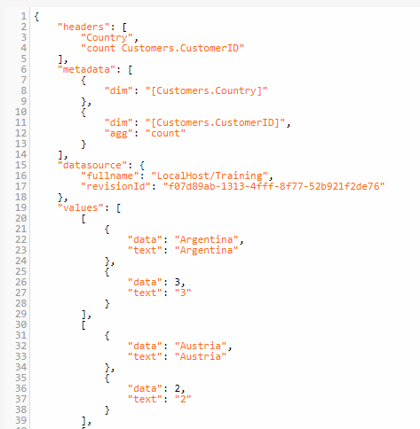
Execute the query, and you should see a result similar to this:

Notice that each member of the values array is an array in itself - and each member of the sub-array is an object containing the value appropriate for one of the metadata items in the query. The first item is a value from the countries dimension, and the second - its corresponding "count of customerID". Thus, the "values" array’s members can be referred to as table rows, and the inner array’s members as each row’s cells, or columns.
# Step 4: Adding a Filter
In this step, you will add a simple filter to the query, so that it returns only countries within the Americas. You will specify the countries you wish to include, so this filter will be applied to the existing dimension in your query ("country").
Add the following property to your "country" metadata object:
"filter": {
    "members": [
        "Argentina", "Canada", "USA",
        "Mexico", "Venezuela", "Brazil"
    ]
}
Note that the filter property is an object, which defines what kind of filtering you want to apply to a dimension. Filter objects can get quite complex, and contain nested JAQL metadata objects. In this case, a filter called "members" is used, which simply defines which values should be included in the query result.
Don’t forget to run the query and ensure the results now only include the countries specified!
# Step 5: Adding a Background Filter
In this stage, you will add another filter to the query - this time, on a dimension that isn’t used in the query. A filter like that is called a "scope filter". This is the type of filter applied by the Sisense UI when filters are added to a widget or dashboard.
You wish to reduce the result set to include only countries in which customers bought Tofu, so you’d like to add a filter for the ProductName dimension, like so:
{
   "dim": "[Products.ProductName]",
   "filter": {
       "members": ["Tofu"]
   }
}
However, if you add this object to the metadata collection you’ll find that it adds another field/column to the query result, "ProductName". If you included more than 1 member in the filter, you’d also find out that results are now grouped by ProductName as well as Country, splitting up your result set in an undesirable manner.
Instead, you’d like to filter the data by this dimension, but not include it in the query at all. To do so, add the following property to the ProductName metadata object:
"panel":"scope"
Run the query now - you should see the result set is now only countries in the Americas where some customers bought Tofu, and a count of such customers for each country.
# Step 6: Adding a Measure Filter
In this step, you will add a filter based on a measure in your query.
You wish to only show countries where more than 1 customer fits the various conditions set up so far. To do so, you will apply a filter to the measure metadata item ("count unique customerID").
Add the following filter object to your measure:
"filter": {
   ">": 1
}
Run the query - you should now see the countries that had only 1 customer disappear from the result set.
# Step 7: Adding a Formula
In this step, you will learn how to add more complex aggregations to your query using formulas.
You will calculate, for each country, the yearly average of orders placed. To do so, you will need a formula like this:
Average of (count unique OrderID) per OrderDate year
As you can see, you will need to use two dimensions in this query (OrderID and OrderDate) as well as one simple aggregation (count unique) and one function (Average with grouping).
Add the following object to your query’s metadata collection:
{
  "formula": "AVG([OrderDateYears], [CountOrderID])",
  "context": {
      "[OrderDateYears]": {
          "dim": "[Orders.OrderDate (Calendar)]",
          "level": "years"
      },
      "[CountOrderID]": {
           "dim": "[Orders.OrderID]",
           "agg": "count"
       }
   }
}
Note that unlike other JAQL metadata items so far, this one does not contain the dim property or any of the other properties you are familiar with. Instead, a formula is composed of two parts: the formulaitself as a string, and a context object to represent various "tokens" found in the formula as JAQL objects.
In this case, the formula uses the AVG function with a dimension to group by, and a numeric measure to apply the average to.
The dimension is represented by the identifier OrderDateYears which is translated to the OrderDate dimension with years level. The measure is represented by the identifier CountOrderID and is translated to the dimension OrderID with the aggregation count applied to it.
Run this query and you should now see 3 cells per each row of your resultset - the third being the result of this formula, calculated for each country.
# Step 8: Using Additional Properties
At this stage, your query should look like this:
{
   "datasource": "Training",
   "metadata": [
       {
           "dim": "[Customers.Country]",
           "filter": {
               "members": [
                   "Argentina", "Canada", "USA",
                   "Mexico", "Venezuela", "Brazil"
               ]
           }
       },
       {
           "dim": "[Customers.CustomerID]",
           "agg": "count",
           "filter": {
               ">":1
           }
       },
       {
           "dim": "[Products.ProductName]",
           "filter": {
               "members": ["Tofu"]
           },
           "panel": "scope"
       },
       {
           "formula": "AVG([OrderDateYears], [CountOrderID])",
           "context": {
               "[OrderDateYears]": {
                   "dim": "[Orders.OrderDate (Calendar)]",
                   "level": "years"
               },
               "[CountOrderID]": {
                   "dim": "[Orders.OrderID]",
                   "agg": "count"
               }
           }
       }
   ]
}
While most of your query building revolves around the metadata property of JAQL, there are some other useful properties you might need. Below are a few of them, which you can add to your query and execute to test them out:
- Try adding the property
"format" : "csv"to the query object’s root (parallel tometadataanddatasource) - executing the query will return data in CSV format, instead of JSON - Try adding the properties
"count": 1and"offset": 0to the query object’s root which will return only the first row. This is useful for paging and lazy-loading of data. - Try adding the property
"sort": "asc"to one of your metadata objects, which will sort the query results by that dimension or measure.
# Part 2: Using JAQL for Custom Filters
In this part of the tutorial, you will utilize your new understanding of JAQL to achieve more advanced filtering on a dashboard, that you wouldn’t otherwise be able to achieve using the Sisense UI.
Open the example dashboard "JAQL-Training-1" attached to this tutorial in order to begin. You will see an empty pivot table and a filter on OrderDate, which is why the pivot is empty. Your goal is to filter the dashboard for data from the last 8 years, which isn’t one of the options in the Time Frame filter UI.
# Step 1: Viewing the JAQL of a Filter
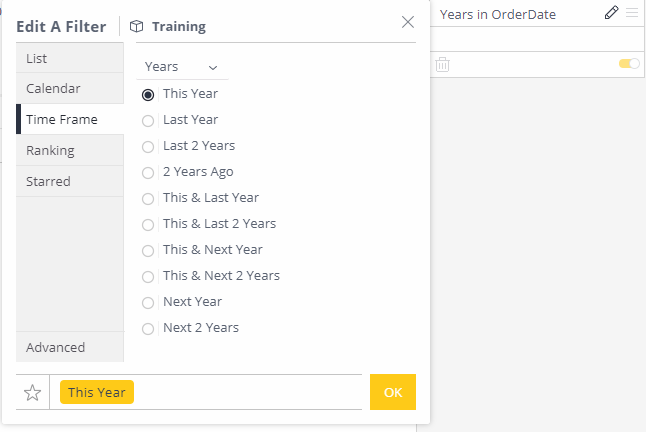
Click the Edit button on the OrderDate dashboard filter:

You can see that the maximum number of years back the UI allows is 2 ("Last 2 Years"), but you would like to increase that range and display data from the past 8 years, for example.
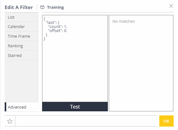
The first stage to do so is finding the JAQL filter created by this UI. Click the Advanced tab, and you will see the following:

Now you can determine the way the filter works via the "last" keyword. JAQL indicates the filter is for past years. "count" and "offset" work exactly as you would expect in the context of paging, and in this case an offset of 0 and count of 1 means data from the current year.
# Step 2: Constructing a Custom Filter
To construct a custom filter, you only need to modify the JAQL extracted from the time frame filter - by changing the "count" property to 8, you will retrieve data from the past 8 years.
However, in some cases you will need to perform a more elaborate modification of the JAQL. For this purpose, the JAQL Reference will be helpful. You can use some capabilities that aren’t present in the UI, such as composite filters using the "and" and "or" keywords.
An important note to remember is that this method applies a filter to a specific dimension, and the Advanced tab only edits the "filter" property of a JAQL metadata object - you cannot combine several dimensions using the "Advanced" tab.
# Step 3: Applying Custom Filters
Use the "Test" button to execute a simple 1 dimensional query using the filter in the "Advanced" tab’s left textbox. You will see up to 10 results, representing which members of the dimension will be retrieved with this filter.
Once you’re satisfied with the result, click OK to create the filter, and it will be applied to the dashboard or widget.
Note that since the filter is a custom one, it has no UI to represent it, and will appear on your filter pane as an empty panel, like so:
# Part 3: Using JAQL Queries in Scripts
In this part of the tutorial, you will learn how to extract the JAQL queries behind various widgets on your dashboard, and a simple method of running JAQL queries from a script and parsing the result.
This is a powerful skill with many different uses - you could execute JAQL yourself for advanced cases of embedding (writing your own visualizations with Sisense data, developing mobile apps with Sisense data), to log or capture the state of various metrics over time, for various automation purposes, and so on.
# Step 1: Extracting JAQL from a widget
Open the attached dashboard called "JAQL-Training-2". You will find an Indicator from which you will extract the underlying JAQL query. Follow these steps:
Edit the widget.
Open your browser’s developer console (usually by pressing F12).
Type in the following code in the console: prism.debugging.GetJaql(prism.activeWidget)
You can now copy the JAQL into a JSON editing tool such as JSON Editor Online (opens new window).
# Step 2: Setting Up and Authentication
Note: This example is written in Node.js. For other languages such as Python, implementation will vary slightly.
Create a new Node.js project, and implement Sisense API authentication by following the instructions in our Using the REST API Tutorial
The Node.js code below is a simple example of this implementation using the request-promise and querystring npm modules.
// Import Modules
const rp = require('request-promise');
const querystring = require('querystring');

/**
* Get Sisense API token
*/
const authenticate = (username, password) => {

   const data = querystring.stringify({
       username,
       password
   });

   const options = {
       url: "https://example.com/api/v1/authentication/login",
       method: "POST",
       headers: {
           "content-type":"application/x-www-form-urlencoded",
           "Content-Length": Buffer.byteLength(data)
       },
       body: data
   };

   return rp(options).then((res) =>{
       const response = JSON.parse(res);
       token = response.access_token;
       return token;
   }).catch((err) => {
       console.error("An error has occurred attempting API call to the authentication/login endpoint.");
       throw err;
   });
}
# Step 3: Executing the Query
The Sisense UI executes JAQL queries via the REST API endpoint:
- On Sisense for Windows: POST /api/elasticubes/{datamodel_title}/jaql
- On Sisense for Linux: POST /api/datasources/{datamodel_title}/jaql
Now that you have extracted a JAQL from an existing widget, you can simply execute it by sending it as the payload. Don’t forget to include the API token retrieved in the previous step.
The Node.js code below is a simple example of a JAQL request to a Sisense for Windows server:
const runJaql = (jaql, cube, token) => {

   const options = {
       url: "https://example.com/api/elasticubes/"+cube+"/jaql",
       method: 'POST',
       headers: {
           "Content-Type": "application/json",
           "Authorization": 'Bearer ' + token
       },
       body: JSON.stringify(jaql);
   };

   return rp(options).then((data) => {
       try {
           return JSON.parse(data);
       }
       catch (e) {
           return data;
       }
   }).catch((err) => {
       console.error("An error has occurred attempting API call to JAQL endpoint.");
       throw err;
   });
}
# Step 4: Parsing the Result
Running the runJaql function from the previous step will return a JavaScript Promise which, if the HTTP call is successful, resolves to a response JSON object which should look like this:
{
   "headers": [
       "Average Orders Per Customer"
   ],
   "datasource": {
       "fullname": "LocalHost/Training",
       "revisionId": "f07d89ab-1313-4fff-8f77-52b921f2de76"
   },
   "metadata": [
       {
           "jaql": {
               "type": "measure",
               "formula": "AVG([99CFE-E7A], [AD2EA-8D0])",
               "context": {
                   "[AD2EA-8D0]": {
                       "table": "Orders",
                       "column": "OrderID",
                       "dim": "[Orders.OrderID]",
                       "datatype": "numeric",
                       "merged": true,
                       "agg": "count",
                       "title": "# of unique OrderID"
                   },
                   "[99CFE-E7A]": {
                       "table": "Customers",
                       "column": "CustomerID",
                       "dim": "[Customers.CustomerID]",
                       "datatype": "text",
                       "merged": true,
                       "title": "CustomerID"
                   }
               },
               "title": "Average Orders Per Customer"
           },
           "format": {
               "mask": {
                   "type": "number",
                   "abbreviations": {
                       "t": true,
                       "b": true,
                       "m": true,
                       "k": false
                   },
                   "separated": true,
                   "decimals": "auto",
                   "isdefault": true
               },
               "color": {
                   "color": "#00cee6",
                   "type": "color"
               }
           },
           "source": "value",
           "handlers": [
               {},
               {}
           ]
       }
   ],
   "values": [
       {
           "data": 4.744186046511628,
           "text": "4.74418604651163"
       }
   ]
}
There are several bits of information you can extract from this response and use in various scenarios, from data sampling, through automation, and up to advanced embedding. Here are a few examples:
- The
valuesproperty contains the actual data (query results). In this case, as the Indicator only returns 1 or 2 measures (numbers) -values[0]andvalues[1]will represent those values. In other cases where dimensions are also involved, the "values" collection will be a matrix (array of arrays) where values[n] represents the n-th row and each object in it is a cell. - The
headersproperty contains an array of table headers, based on the various JAQL object’s titles or dimensions. It can help you discern which object represents which "column" and in rendering the results into a UI or other data format, such as CSV. - The
metadataproperty contains metadata on the query results - JAQL objects representing the various columns in the result set. Note that it does not contain all of the fields in the query - only those that end up in the result set. It contains useful information such as each column’s unique formatting configuration.